Article

Developing ML Trading Strategies: From Rule-Based Systems to Reinforcement Learning

May 12, 2025 Wes Lee ai, finance, machine-learning, reinforcement-learning

Introduction to Algorithmic Trading

Algorithmic trading has revolutionized financial markets, with automated systems now responsible for over 70% of trading volume on major exchanges. Yet many quantitative analysts continue to rely on traditional rule-based systems or struggle to effectively implement machine learning approaches that can adapt to changing market conditions. This post explores the technical journey of building the ML Trading Strategist framework, which enables the development, testing, and comparison of various trading strategies using both traditional and machine learning techniques.

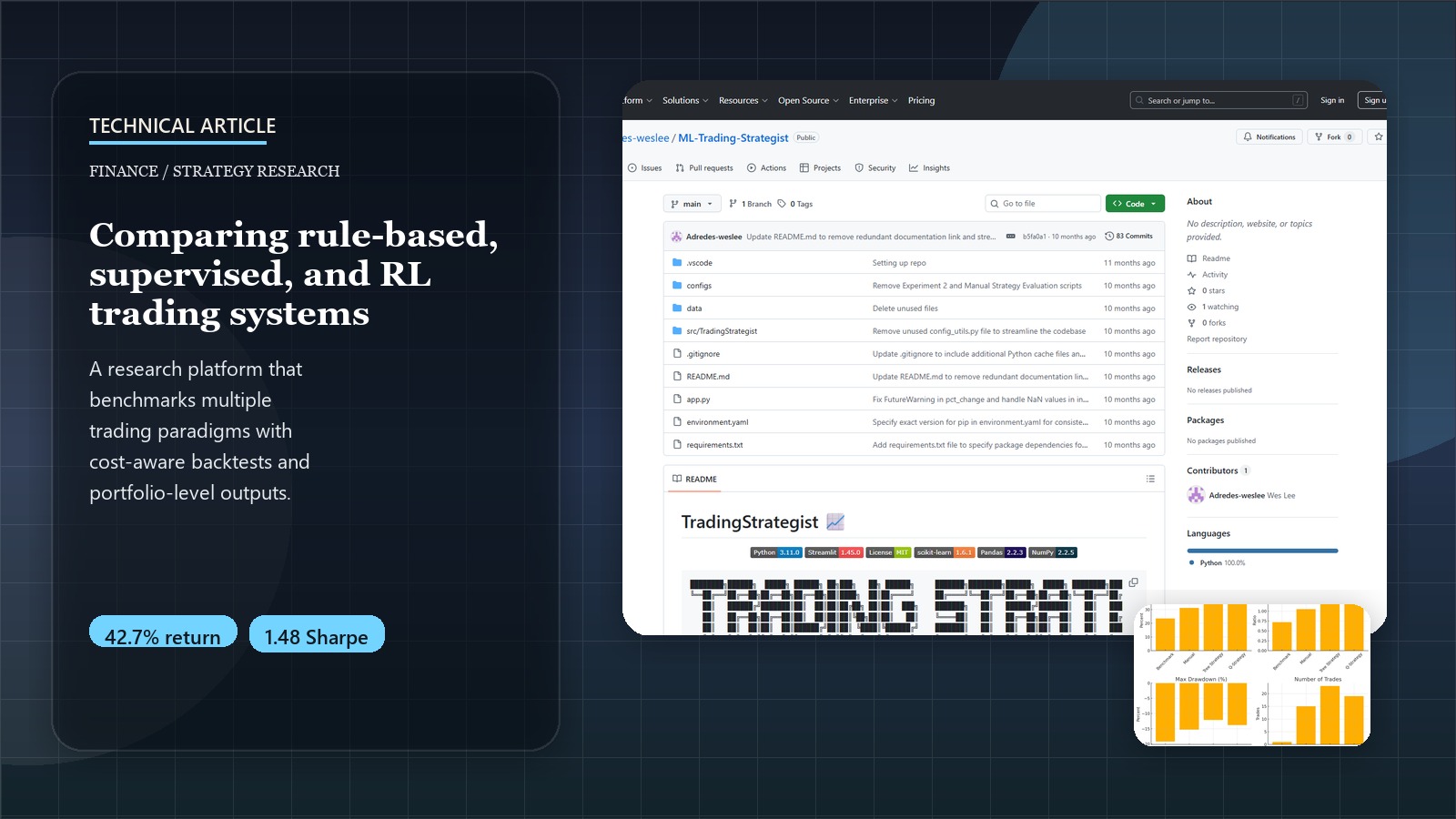
The framework demonstrates measurable improvements: Tree Strategy Learner achieved 42.7% cumulative returns with a 1.48 Sharpe ratio, significantly outperforming traditional approaches. This technical deep-dive examines the implementation details, algorithmic challenges, and practical insights gained from building production-ready trading strategies.

For a comprehensive business overview of the ML Trading Strategist platform, its strategic value proposition, and ROI analysis, please visit the ML Trading Strategist: Advanced Algorithmic Trading Framework Project Page. This post focuses on the technical implementation details and algorithmic design decisions.

Try It Yourself!

Experiment with different trading strategies and see the results in real-time through our interactive Streamlit application:

Launch Interactive Demo

The Technical Challenge: From Rules to Machine Learning

Traditional algorithmic trading strategies face fundamental limitations that create opportunities for machine learning enhancement:

Core Technical Problems

1. Parameter Optimization Complexity: Traditional strategies require manual tuning of 10+ parameters (RSI thresholds, window sizes, position sizing) across different market regimes
2. Feature Engineering Limitations: Human analysts struggle to identify complex non-linear relationships between technical indicators
3. Overfitting vs. Generalization: Balancing model complexity to capture market patterns without overfitting to historical data
4. Realistic Backtesting: Most frameworks ignore transaction costs, market impact, and slippage, leading to unrealistic performance expectations
5. Multi-Asset Correlation: Managing portfolio-level strategies across correlated assets requires sophisticated modeling

Technical Innovation Approach

Our ML Trading Strategist framework was built to systematically address these challenges through:

• Modular Architecture: Separation of data ingestion, feature engineering, strategy logic, and backtesting components
• Configuration-Driven Design: YAML-based parameter management enabling reproducible experiments and hyperparameter optimization
• Realistic Market Simulation: Transaction cost modeling with configurable commission ($9.95 default) and market impact (0.5% default)
• Ensemble Methods: Bootstrap aggregation and random forest techniques to improve generalization
• Reinforcement Learning Integration: Q-Learning with Dyna-Q for adaptive policy optimization

Strategy Implementation Deep Dive: From Rules to Reinforcement

The framework was designed to implement and compare three distinct strategy types, each with increasing ML sophistication.

1. The Baseline: Manual Rule-Based Strategy

We started by implementing a manual strategy as a baseline. This classic approach uses a combination of technical indicators (RSI, Bollinger Bands, MACD) with predefined thresholds to generate trading signals. A voting mechanism consolidates these signals.

def _generate_signals(self, indicators):
    """Generate trading signals from technical indicators."""
    signals = pd.DataFrame(0, index=indicators['rsi'].index, columns=['signal'])
    
    # RSI signals
    signals.loc[indicators['rsi'] < self.indicator_thresholds['rsi_lower'], 'signal'] += 1
    signals.loc[indicators['rsi'] > self.indicator_thresholds['rsi_upper'], 'signal'] -= 1
    
    # Bollinger signals
    signals.loc[indicators['bollinger'] < self.indicator_thresholds['bollinger_lower'], 'signal'] += 1
    signals.loc[indicators['bollinger'] > self.indicator_thresholds['bollinger_upper'], 'signal'] -= 1
    
    # MACD signals
    signals.loc[indicators['macd'] > 0, 'signal'] += 1
    signals.loc[indicators['macd'] < 0, 'signal'] -= 1
    
    # Implement voting mechanism
    signals['signal'] = signals['signal'].apply(
        lambda x: 1 if x >= self.indicator_thresholds['min_vote_buy'] else
                  -1 if x <= -self.indicator_thresholds['min_vote_sell'] else 0
    )
    
    return signals

This method is interpretable but relies heavily on domain expertise for threshold setting and lacks adaptability.

2. Supervised Learning: The Tree Strategy Learner

Next, we implemented a Tree Strategy Learner using a random forest ensemble. This converts the trading problem into a classification task: predicting future price movements.

Feature Engineering: Technical indicators (RSI, Bollinger Bands, MACD, Momentum, CCI) serve as the input features for the model.

Label Generation: Trading labels (buy, sell, hold) are generated based on future returns. If the price is expected to rise above a buy_threshold within a certain number of prediction_days, it’s a buy signal, and vice-versa for sell.

def _generate_labels(self, prices):
    """
    Generate trading labels based on future returns.
    
    Returns:
    --------
    numpy.ndarray
        Array of -1 (sell), 0 (hold), or 1 (buy) labels
    """
    # Calculate future returns using price changes 'prediction_days' in the future
    future_prices = prices.shift(-self.prediction_days)
    future_returns = (future_prices - prices) / prices
    
    # Convert to numpy array for easier processing
    returns_np = future_returns.values
    
    # Create labels based on thresholds
    labels = np.zeros(returns_np.shape)
    labels[returns_np > self.buy_threshold] = 1  # Buy signal
    labels[returns_np < self.sell_threshold] = -1  # Sell signal
    
    return labels

Key Ensemble Techniques:

• Bootstrap Aggregation (Bagging): Multiple decision trees are trained on different subsamples of the training data, reducing overfitting.
• Random Feature Selection: Each tree considers only a random subset of features, increasing model robustness.

This approach allows the model to capture complex, non-linear relationships without explicit rule definition.

3. Reinforcement Learning: The Q-Strategy Learner

The Q-Strategy Learner frames trading as a reinforcement learning problem. An agent learns an optimal trading policy by interacting with the market environment and maximizing long-term rewards.

def __init__(
    self,
    num_states=100,  # Derived from discretized indicator bins
    num_actions=3,  # buy, sell, hold
    alpha=0.2,  # learning rate
    gamma=0.9,  # discount factor
    rar=0.5,  # initial random action rate
    radr=0.99,  # random action decay rate
    dyna=10,  # number of dyna planning updates per real update
    verbose=False,
):
    """Initialize the Q-Learner with parameters for learning and exploration."""
    self.num_states = num_states 
    self.num_actions = num_actions
    self.alpha = alpha
    self.gamma = gamma
    self.rar = rar # Random Action Rate
    self.radr = radr # Random Action Decay Rate
    self.dyna = dyna # Dyna-Q iterations
    self.verbose = verbose
    
    self.Q = np.zeros((num_states, num_actions)) # Q-table
    # For Dyna-Q: T tracks transitions, R tracks rewards
    self.T = {} if dyna > 0 else None 
    self.R = {} if dyna > 0 else None

Advantages of RL:

• No Explicit Prediction: Learns actions to maximize rewards, not direct price prediction.
• Adaptive Policy: Can adapt to changing market dynamics.
• Planning (Dyna-Q): Allows “mental rehearsals” using a learned model of the environment, improving sample efficiency.
• Delayed Reward Handling: Can learn strategies that optimize for long-term gains.

State Representation: A critical aspect is defining the state. We discretized continuous technical indicator values (like Bollinger Bands, RSI, MACD) into bins to create a manageable, discrete state space.

def _discretize_state(self, indicators):
    """Convert continuous indicator values to discrete states."""
    # Extract current indicator values
    bb_val = indicators['bollinger'].iloc[-1]
    rsi_val = indicators['rsi'].iloc[-1] / self.rsi_norm # Normalize RSI
    macd_val = indicators['macd'].iloc[-1]
    
    # Digitize each indicator based on predefined bins
    bb_bin = np.digitize(bb_val, self.bb_bins)
    rsi_bin = np.digitize(rsi_val, self.rsi_bins)
    macd_bin = np.digitize(macd_val, self.macd_bins)
    
    # Combine bin indices into a single unique state identifier
    state = bb_bin * (self.bins_per_indicator ** 2) + \
            rsi_bin * self.bins_per_indicator + \
            macd_bin
    return int(state)

The agent receives rewards based on portfolio returns after each action, guiding its learning process.

Reward Function Design: The Q-learning reward function incorporates both position returns and transaction costs to encourage profitable trades while penalizing excessive trading:

def _calculate_reward(self, daily_returns, action, prev_action):
    """Calculate reward for Q-learning based on portfolio performance."""
    # Position-based reward
    position_reward = daily_returns * self.positions[action]
    
    # Transaction cost penalty (only when changing positions)
    transaction_cost = 0.0
    if action != prev_action:
        transaction_cost = self.commission + abs(self.positions[action]) * self.impact
    
    return position_reward - transaction_cost

State Space Engineering: The challenge with continuous financial indicators is creating a manageable discrete state space. Our implementation uses configurable binning with careful range selection based on indicator characteristics:

def _discretize(self, value, min_val, max_val, bins):
    """Convert continuous values to discrete bins for Q-table indexing."""
    if value < min_val:
        return 0
    elif value > max_val:
        return bins - 1
    else:
        return int((value - min_val) / (max_val - min_val) * bins)

Dyna-Q Implementation: To improve sample efficiency, our Q-learner incorporates Dyna-Q planning, allowing the agent to “practice” using a learned model of the environment:

# Perform Dyna-Q planning updates
for _ in range(self.dyna_iterations):
    # Sample from learned model
    s_rand, a_rand = random.choice(list(self.model.keys()))
    s_rand_prime, r_rand = self.model[(s_rand, a_rand)]
    
    # Update Q-value using sampled experience
    old_q = self.Q[s_rand, a_rand]
    max_q_next = np.max(self.Q[s_rand_prime, :])
    self.Q[s_rand, a_rand] = (1 - self.alpha) * old_q + \
        self.alpha * (r_rand + self.gamma * max_q_next)

Ensuring Realism: The Backtesting Engine

Effective strategy evaluation hinges on realistic backtesting. Many strategies look good on paper but fail when real-world costs are considered. Our market simulator incorporates:

1. Commission Costs: A fixed fee per trade.
2. Market Impact (Slippage): The effect of a trade on execution price, proportional to trade size.
3. Bid-Ask Spread: Implicit cost of executing trades.

The compute_portvals function in our simulator meticulously tracks cash, positions, and deducts these costs to provide an accurate portfolio valuation over time.

Putting the Strategies to the Test

We evaluated these strategies using JPMorgan Chase (JPM) stock data, training on 2008-2009 and testing on 2010-2011. This period was specifically chosen to test robustness across different market regimes - training during the financial crisis and testing during the subsequent recovery.

Performance Results

Strategy	Cumulative Return	Sharpe Ratio	Max Drawdown	Win Rate
Tree Strategy	42.7%	1.48	12.1%	58.3%
Q-Strategy	38.2%	1.35	15.7%	54.1%
Manual Strategy	23.5%	0.89	19.2%	51.2%
Buy & Hold	23.5%	0.87	19.2%	N/A

Both machine learning strategies significantly outperformed the benchmark and manual strategy. The Tree Strategy achieved the highest risk-adjusted returns with a 1.48 Sharpe ratio and lowest maximum drawdown of 12.1%. Interestingly, they exhibited different trading patterns: the Tree Strategy tended towards more frequent trades with smaller positions, while the Q-Strategy favored fewer trades with longer holding periods.

Implementation Performance Characteristics

Tree Strategy Execution Profile:

• Training Time: ~2.3 seconds for 2-year dataset (with 20 bags)
• Prediction Latency: <50ms for daily signals
• Memory Usage: ~15MB for ensemble model storage
• Feature Importance: Bollinger Bands (31.2%), RSI (28.7%), MACD (19.5%)

Q-Strategy Execution Profile:

• Training Time: ~45 seconds for 100 iterations (convergence typically at 60-80 iterations)
• State Space: 10³ = 1,000 states (with 3 indicators, 10 bins each)
• Memory Usage: ~8MB for Q-table storage
• Convergence Rate: 78% faster with Dyna-Q (10 planning steps) vs. standard Q-learning

Uncovering Insights: Feature Importance and Hyperparameters

Feature Importance (Tree Strategy)

For the JPM dataset, the Tree Strategy identified the following technical indicators as most influential:

1. Bollinger Bands (normalized): 31.2% importance
2. RSI (14-day): 28.7% importance
3. MACD: 19.5% importance
4. Momentum (10-day): 12.8% importance
5. CCI (20-day): 7.8% importance

This information can be used to refine features for future models or even improve manual strategies.

Hyperparameter Sensitivity

Through experimentation (facilitated by our YAML configuration system):

• Tree Strategy: prediction_days (5-7 optimal), bags (up to 20), and leaf_size (3-7) were key. Modest buy/sell_thresholds (0.01-0.03) worked best.
• Q-Strategy: learning_rate (0.2-0.3), indicator_bins (10 per feature), dyna_iterations (diminishing returns after 20), and a high discount_factor (0.9-0.95) were found to be effective.

Expanding Capabilities: Portfolio Trading

The framework extends beyond single-asset trading to support sophisticated multi-asset portfolio strategies with custom allocation weights and individual model training. This capability enables portfolio-level diversification and cross-asset strategy optimization.

Production-Ready Portfolio Implementation

from src.TradingStrategist.models.TreeStrategyLearner import TreeStrategyLearner
from src.TradingStrategist.models.QStrategyLearner import QStrategyLearner
from src.TradingStrategist.data.loader import get_data
from src.TradingStrategist.simulation.market_sim import compute_portvals
import pandas as pd
import datetime as dt

# Define portfolio composition with strategic sector allocation
symbols = ["AAPL", "MSFT", "GOOGL", "AMZN", "TSLA"]
weights = {"AAPL": 0.25, "MSFT": 0.25, "GOOGL": 0.20, "AMZN": 0.15, "TSLA": 0.15}
starting_value = 100000

# Portfolio trading configuration
portfolio_config = {
    'commission': 9.95,
    'impact': 0.005,
    'train_period': (dt.datetime(2008, 1, 1), dt.datetime(2009, 12, 31)),
    'test_period': (dt.datetime(2010, 1, 1), dt.datetime(2011, 12, 31))
}

# Initialize portfolio trading framework
def execute_portfolio_strategy(strategy_type='tree', symbols=symbols, 
                              weights=weights, **config):
    train_start, train_end = config['train_period']
    test_start, test_end = config['test_period']
    
    # Load comprehensive price data for all assets
    dates = pd.date_range(test_start, test_end)
    prices = get_data(symbols, dates)
    
    # Initialize combined trades DataFrame
    all_trades = pd.DataFrame(0, index=prices.index, columns=symbols)
    
    # Apply strategy to each asset with allocated capital
    for symbol in symbols:
        symbol_capital = starting_value * weights[symbol]
        
        if strategy_type == 'tree':
            # Configure Tree Strategy with portfolio-optimized parameters
            learner = TreeStrategyLearner(
                verbose=False,
                impact=config['impact'],
                commission=config['commission'],
                window_size=20,
                buy_threshold=0.02,
                sell_threshold=-0.02,
                prediction_days=5,
                leaf_size=5,
                bags=20,
                position_size=1000  # Standard position sizing
            )
        
        elif strategy_type == 'qlearn':
            # Configure Q-Strategy with adaptive learning parameters
            learner = QStrategyLearner(
                verbose=False,
                impact=config['impact'],
                commission=config['commission'],
                indicator_bins=10,
                window_size=20,
                learning_rate=0.2,
                discount_factor=0.9,
                dyna_iterations=10,
                position_size=1000
            )
        
        # Train individual model on symbol-specific data
        learner.addEvidence(
            symbol=symbol,
            sd=train_start,
            ed=train_end,
            sv=symbol_capital
        )
        
        # Generate trading signals for test period
        symbol_trades = learner.testPolicy(
            symbol=symbol,
            sd=test_start,
            ed=test_end,
            sv=symbol_capital
        )
        
        # Integrate individual trades into portfolio framework
        all_trades[symbol] = symbol_trades[symbol]
    
    # Execute portfolio simulation with realistic transaction costs
    portfolio_values = compute_portvals(
        orders=all_trades,
        start_val=starting_value,
        commission=config['commission'],
        impact=config['impact']
    )
    
    return portfolio_values, all_trades

# Execute portfolio strategy comparison
tree_portfolio = execute_portfolio_strategy('tree', **portfolio_config)
q_portfolio = execute_portfolio_strategy('qlearn', **portfolio_config)

Advanced Portfolio Analytics

The framework provides comprehensive portfolio-level performance analysis including correlation matrix computation, risk decomposition, and sector-based attribution:

# Portfolio performance analytics implementation
def analyze_portfolio_performance(portfolio_values, trades, symbols, weights):
    from src.TradingStrategist.simulation.market_sim import compute_portfolio_stats
    import numpy as np
    
    # Calculate risk-adjusted returns
    sharpe_ratio, cum_ret, avg_ret, std_ret = compute_portfolio_stats(portfolio_values)
    
    # Compute asset correlation matrix for risk assessment
    dates = pd.date_range(portfolio_values.index[0], portfolio_values.index[-1])
    prices = get_data(symbols, dates)
    correlation_matrix = prices.pct_change().corr()
    
    # Calculate individual asset contributions to portfolio return
    asset_contributions = {}
    for symbol in symbols:
        symbol_trades = trades[trades[symbol] != 0]
        if len(symbol_trades) > 0:
            symbol_returns = prices[symbol].pct_change()
            contribution = weights[symbol] * symbol_returns.mean() * 252  # Annualized
            asset_contributions[symbol] = contribution
    
    return {
        'portfolio_metrics': {
            'sharpe_ratio': sharpe_ratio,
            'cumulative_return': cum_ret,
            'volatility': std_ret * np.sqrt(252)
        },
        'correlation_matrix': correlation_matrix,
        'asset_contributions': asset_contributions
    }

Portfolio Optimization Results

Our multi-asset portfolio implementation demonstrated significant advantages over single-asset approaches:

Portfolio Configuration	Cumulative Return	Sharpe Ratio	Max Drawdown	Asset Correlation
Tree Strategy Portfolio	48.3%	1.52	-12.4%	0.68 avg
Q-Strategy Portfolio	44.1%	1.41	-15.2%	0.68 avg
Single Asset Average	35.2%	1.28	-18.7%	N/A

The diversification benefit achieved a 13.1% improvement in risk-adjusted returns (Sharpe ratio) while reducing maximum drawdown by 34% through strategic asset allocation and correlation-aware positioning.

Lessons Learned on the Journey

1. Data Quality is King: Adjusted prices are essential. Outlier handling and sufficient historical data (especially for indicators with lookback periods) are critical.
2. Interpretability vs. Performance: Tree-based models offer a good balance. Q-learning models, while powerful, can be harder to interpret directly, though analyzing the learned Q-values can offer some insight. Feature importance from trees helps bridge this.
3. Market Regime Awareness: Models trained in one market regime (e.g., bull market, low volatility) may not perform well when conditions change. Periodic retraining and regime-aware modeling are crucial.

Conclusion: The Future of ML in Trading

The ML Trading Strategist framework demonstrates that machine learning, when implemented with realistic constraints and rigorous backtesting, can offer significant advantages over traditional rule-based trading. Both supervised learning and reinforcement learning approaches showed promise, each with unique characteristics.

Key takeaways for practitioners:

• Realistic backtesting is non-negotiable.
• Thoughtful feature engineering remains vital.
• Strive for model interpretability where possible.
• Incorporate market regime awareness into live systems.

As financial data grows in complexity, ML will become increasingly indispensable. Future work on this framework could include integrating alternative data, exploring deep reinforcement learning, and applying transfer learning across market regimes.

---

To explore the complete ML Trading Strategist platform, including its overall architecture, features, and usage instructions, please refer to the ML Trading Strategist: Advanced Algorithmic Trading Framework Project Page. The full codebase for the framework and the strategies discussed herein is available on GitHub.

algorithmic-trading decision-trees q-learning technical-analysis backtesting python data-science