Article
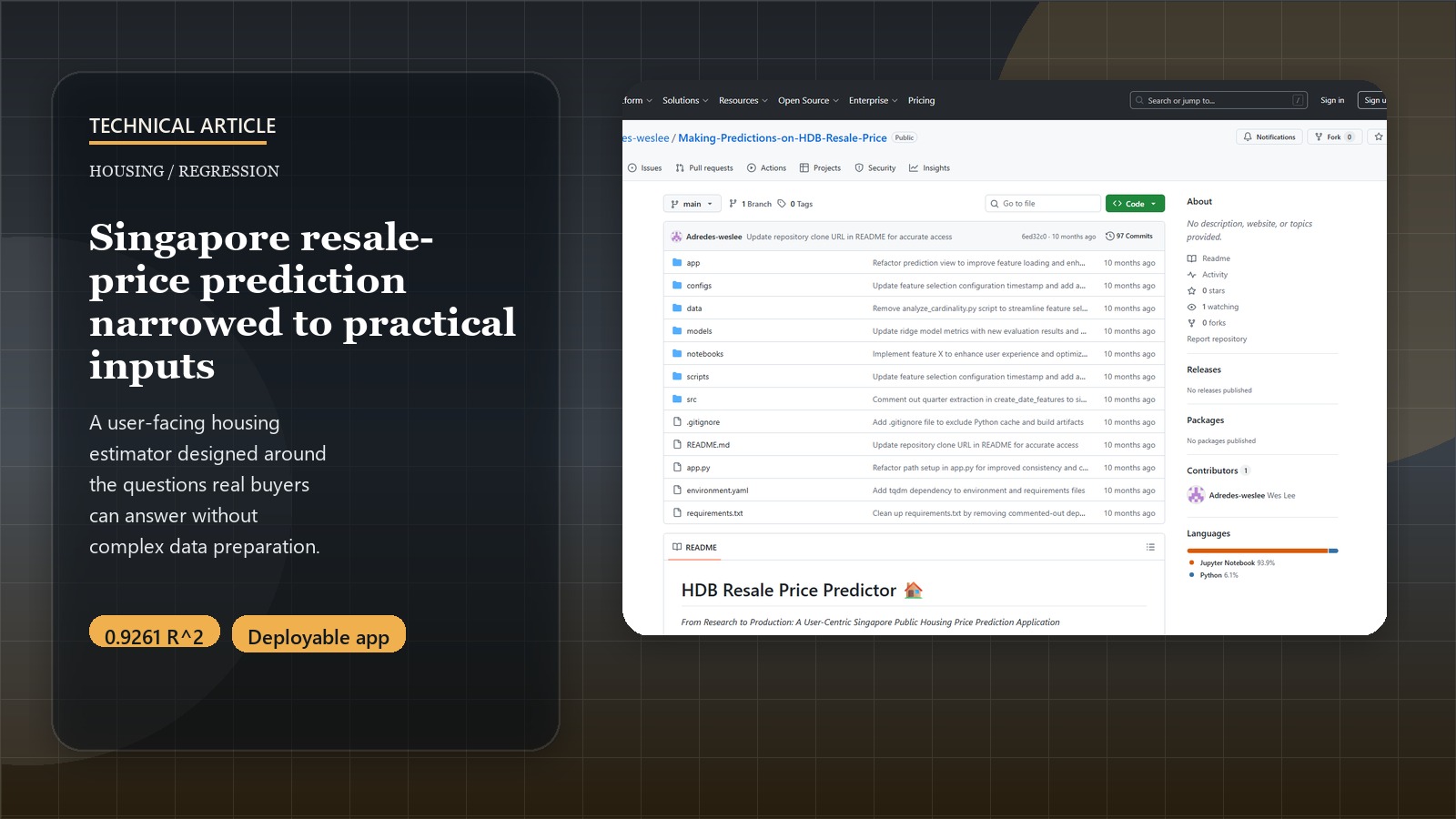
Building an HDB Resale Price Predictor: A Technical Deep Dive into Feature Engineering and Regression
Introduction: Decoding Singapore’s Unique Housing Market with Data
Singapore’s public housing (HDB flats) market is a dominant feature of its urban landscape, housing over 80% of the population. Predicting HDB resale prices is not just an academic exercise; it has significant financial implications for citizens and provides valuable insights for urban planning. This post offers a technical walkthrough of a project that evolved from academic research to a production-ready application, detailing the data processing, feature engineering, modeling techniques, and architectural decisions that enable real-world deployment.
For a higher-level overview of this project’s significance, key findings, and policy implications for Singapore, please see the HDB Resale Price Insights: A Data-Driven Analysis for Singapore’s Housing Market Project Page.
Predict HDB Resale Prices!
Experience the production application built from this technical implementation:
Launch Price PredictorThe Technical Architecture: From Research to Production
This project underwent a significant evolution from academic research to production deployment. Understanding this transformation is crucial to appreciating the technical decisions made.
Project Evolution Journey
Phase 1: Research Foundation (notebooks/making_predictions_on_HDB_resale_price.ipynb)
- Comprehensive EDA with 150+ engineered features
- Academic rigor: Statistical significance testing, multicollinearity analysis
- Maximum accuracy focus: 92.78% R² score with complex feature engineering
Phase 2: Production Transformation (Current architecture)
- User-centric design: Streamlined to essential, user-providable features
- Pipeline-first approach: Consistent preprocessing for training and inference
- Deployment-ready: Modular architecture supporting both local and cloud deployment
Production Architecture
├── app.py                  # Main Streamlit application entry point
├── app/                    # Streamlit application modules
│   ├── components/        # Reusable UI components (sidebar, visualizations)
│   ├── pages/             # Individual page modules
│   ├── views/             # Core view components (home, prediction, insights)
│   └── main.py            # Application routing and configuration
├── src/                   # Core business logic
│   ├── data/              # Data loading, preprocessing, and feature engineering
│   ├── models/            # Prediction models, training, and evaluation
│   ├── utils/             # Helper functions and utilities
│   └── visualization/     # Plotting and mapping utilities
├── models/                # Trained model artifacts (.pkl files and metadata)
├── configs/               # Configuration files (YAML, JSON)
├── scripts/               # Training and utility scripts
└── requirements.txt       # Python 3.11 dependencies
The Data Science Implementation: Technical Deep Dive
Our goal was to build an accurate, interpretable, and production-deployable model for HDB resale prices. This involved several key technical stages.
1. Dataset Architecture and Processing Pipeline
The production system uses a structured data pipeline with multiple sources:
Primary Dataset: Kaggle HDB resale dataset (60,000+ transactions)
# Data loading implementation
from src.data.loader import load_training_data, load_raw_data

# Load raw data with validation
raw_df = load_raw_data("data/raw/kaggle_hdb_df.csv")
X, y = load_training_data("data/processed/train_pipeline_processed.csv")
Data Structure:
- Raw data:
data/raw/- Original transaction records - Processed data:
data/processed/- Feature-engineered datasets - Pipeline splits: Separate exploratory and production preprocessing paths
Key Columns:
# Core features from actual implementation
numerical_features = [
    "lease_commence_date", "Tranc_Year", "Tranc_Month",
    "mid_storey", "hdb_age", "max_floor_lvl",
    "total_dwelling_units", "floor_area_sqm"
]

categorical_features = [
    "town", "flat_type", "flat_model", "storey_range"
]
2. Production-Ready Feature Engineering Pipeline
The feature engineering system is built using modular, reusable components that ensure consistency between training and inference.
a. Temporal Feature Engineering:
# From src/data/preprocessing_pipeline.py
def create_date_features(df: pd.DataFrame) -> pd.DataFrame:
    """Create temporal features from transaction date."""
    df_copy = df.copy()

    if 'Tranc_YearMonth' in df_copy.columns:
        # Extract temporal components
        df_copy['Tranc_Year'] = df_copy['Tranc_YearMonth'].dt.year
        df_copy['Tranc_Month'] = df_copy['Tranc_YearMonth'].dt.month
        df_copy['Tranc_Quarter'] = df_copy['Tranc_YearMonth'].dt.quarter

        # Calculate HDB age at transaction
        df_copy['hdb_age'] = df_copy['Tranc_Year'] - df_copy['lease_commence_date']

        # Remaining lease calculations
        df_copy['remaining_lease_years'] = df_copy['lease_commence_date'] + 99 - df_copy['Tranc_Year']

        # Critical lease decay thresholds
        df_copy['lease_lt_60_years'] = (df_copy['remaining_lease_years'] < 60).astype(int)
        df_copy['lease_lt_40_years'] = (df_copy['remaining_lease_years'] < 40).astype(int)

    return df_copy
b. Storey and Spatial Features:
# From actual implementation - storey range processing
def process_storey_features(df: pd.DataFrame) -> pd.DataFrame:
    """Convert storey range to numerical features."""
    df_copy = df.copy()

    # Extract storey range bounds
    df_copy['lower'] = df_copy['storey_range'].str.extract('(\d+)').astype(float)
    df_copy['upper'] = df_copy['storey_range'].str.extract('TO (\d+)').astype(float)
    df_copy['mid_storey'] = (df_copy['lower'] + df_copy['upper']) / 2

    return df_copy
c. Configuration-Driven Feature Selection:
# From configs/model_config.yaml
features:
  categorical_encoding: "one-hot"
  scaling: "standard"
  feature_selection:
    enabled: true
    method: "f_regression"  # or "mutual_info_regression"
    percentile: 99
d. Lease Decay Feature Engineering:
# Advanced lease feature engineering
def create_lease_features(df: pd.DataFrame) -> pd.DataFrame:
    """Create comprehensive lease-based features."""
    df_copy = df.copy()

    # Calculate remaining lease in years at the time of transaction
    # HDB leases are typically 99 years
    df_copy['remaining_lease_years'] = df_copy['lease_commence_year'] + 99 - df_copy['transaction_year']

    # Create binary indicators for critical lease decay thresholds
    # Research and market observations suggest price impacts at these points
    df_copy['lease_lt_60_years'] = (df_copy['remaining_lease_years'] < 60).astype(int)
    df_copy['lease_lt_40_years'] = (df_copy['remaining_lease_years'] < 40).astype(int)

    # Calculate percentage of lease remaining
    df_copy['lease_remaining_percentage'] = df_copy['remaining_lease_years'] / 99.0

    # Interaction term: floor area * remaining lease (value per sqm might change with lease)
    if 'floor_area_sqm' in df_copy.columns:
        df_copy['floor_area_x_rem_lease_pct'] = df_copy['floor_area_sqm'] * df_copy['lease_remaining_percentage']

    return df_copy

# Example usage:
hdb_data_with_lease_features = create_lease_features(hdb_raw_data)
print(hdb_data_with_lease_features[['remaining_lease_years', 'lease_lt_60_years', 'lease_remaining_percentage']].head())
This captures the non-linear impact of lease decay, where depreciation often accelerates as the lease shortens, particularly below key thresholds like 60 or 40 years remaining.
e. Location and Proximity Features: Location is paramount. Beyond just the ‘town’, we would ideally engineer features like:
- Distance to the nearest MRT station.
- Distance to Central Business District (CBD).
- Number of schools within a certain radius (e.g., 1km, 2km).
- Proximity to shopping malls and other key amenities. (These often require joining with external geospatial datasets or using APIs, which was abstracted in the original project description but is a key step).
f. Flat Characteristics:
- Storey Level: Convert storey range (e.g., “01 TO 03”, “10 TO 12”) to an average numerical value or ordinal encoding. Higher floors generally command higher prices.
- Flat Type and Model: One-hot encode or use target encoding for categorical variables like
flat_type(e.g., ‘3 ROOM’, ‘4 ROOM’, ‘EXECUTIVE’) andflat_model(e.g., ‘Model A’, ‘DBSS’, ‘Improved’).
3. Data Preprocessing: Preparing Data for Modeling
Robust preprocessing is essential for model performance and stability.
- Handling Missing Values: For features with missing data,
IterativeImputerfrom Scikit-learn was used. This is an advanced imputer that models each feature with missing values as a function of other features, and uses that estimate for imputation.from sklearn.experimental import enable_iterative_imputer # Enable experimental feature from sklearn.impute import IterativeImputer # Assuming X_train_numeric is your training data with only numeric features # imputer = IterativeImputer(max_iter=10, random_state=0) # X_train_numeric_imputed = imputer.fit_transform(X_train_numeric) # X_test_numeric_imputed = imputer.transform(X_test_numeric) # Use transform on test data - Categorical Variable Encoding:
- For nominal categorical features (like
townorflat_modelif no inherent order), One-Hot Encoding is common. - For ordinal features (like
storey_rangeif converted to ordered categories), Ordinal Encoding can be used. - The project mentioned Polynomial Encoding, which can capture interactions between categorical features but can lead to a high number of features.
- For nominal categorical features (like
- Feature Scaling: Numerical features were standardized using
StandardScalerto bring them to a similar scale, which is important for many regression algorithms, especially those with regularization.from sklearn.preprocessing import StandardScaler # scaler = StandardScaler() # X_train_scaled = scaler.fit_transform(X_train_numeric_imputed) # Fit on train, then transform # X_test_scaled = scaler.transform(X_test_numeric_imputed) # Transform test - Multicollinearity Analysis: Variance Inflation Factor (VIF) analysis was conducted to identify and potentially remove or combine highly correlated features, which can destabilize linear models.
- Feature Selection:
- Mutual Information: To assess the relationship between each feature and the target variable (resale price).
- LASSO Regularization: Used not only for modeling but also implicitly for feature selection, as it tends to shrink coefficients of less important features to zero.
4. Production Model Development: Pipeline-Based Approach
The production system implements a comprehensive pipeline approach that ensures consistency and reproducibility across training and deployment.
a. Model Architecture:
# From src/models/training.py - Actual implementation
MODEL_TYPES = {
    'linear': LinearRegression,
    'ridge': Ridge,
    'lasso': Lasso
}

def train_and_save_pipeline_model(model_type='linear', data_path=None):
    """Train a complete model pipeline including preprocessing."""

    # Load data
    df = pd.read_csv(data_path)
    X = df.drop(['resale_price'], axis=1)
    y = df['resale_price']

    # Create preprocessing pipeline
    preprocessor = create_standard_preprocessing_pipeline()

    # Create complete pipeline
    pipeline = Pipeline([
        ('preprocessor', preprocessor),
        ('model', MODEL_TYPES[model_type]())
    ])

    # Split data for validation
    X_train, X_val, y_train, y_val = train_test_split(
        X, y, test_size=0.2, random_state=42
    )

    # Train pipeline
    pipeline.fit(X_train, y_train)

    # Evaluate performance
    train_score = pipeline.score(X_train, y_train)
    val_score = pipeline.score(X_val, y_val)
    y_pred = pipeline.predict(X_val)
    rmse = np.sqrt(mean_squared_error(y_val, y_pred))

    # Save complete pipeline
    model_path = f'models/pipeline_{model_type}_model.pkl'
    joblib.dump(pipeline, model_path)

    return {
        'pipeline': pipeline,
        'metrics': {
            'train_r2': train_score,
            'val_r2': val_score,
            'rmse': rmse
        }
    }
b. Streamlit Application Integration:
# From app/views/prediction.py - Real-time prediction
@st.cache_resource
def load_model():
    """Load the trained pipeline model."""
    try:
        # Try multiple model paths for flexibility
        model_paths = [
            'models/pipeline_ridge_model.pkl',
            'models/pipeline_linear_model.pkl',
            'models/pipeline_lasso_model.pkl'
        ]

        for path in model_paths:
            if os.path.exists(path):
                return joblib.load(path)

    except Exception as e:
        st.error(f"Error loading model: {e}")
        return None

def make_prediction(model, user_input):
    """Generate price prediction from user input."""

    # Process user input through feature engineering
    processed_input = process_user_input(user_input)

    # Make prediction using the complete pipeline
    prediction = model.predict(processed_input)[0]

    # Get prediction confidence interval
    prediction_std = model.named_steps['model'].predict(
        model.named_steps['preprocessor'].transform(processed_input)
    ).std() if hasattr(model.named_steps['model'], 'predict') else 0

    return {
        'predicted_price': prediction,
        'confidence_interval': prediction_std * 1.96,  # 95% CI
        'price_per_sqm': prediction / user_input['floor_area_sqm']
    }
c. Configuration-Driven Training:
# From configs/model_config.yaml - Production configuration
model:
  type: "ridge"  # linear, ridge, or lasso
  hyperparameters:
    alpha: 1.0  # Regularization strength
    max_iter: 1000
    random_state: 42

preprocessing:
  categorical_encoding: "onehot"
  numerical_scaling: "standard"
  handle_unknown: "ignore"

validation:
  test_size: 0.2
  cv_folds: 5
  scoring: ["r2", "neg_mean_squared_error"]

features:
  numerical:
    - "floor_area_sqm"
    - "hdb_age"
    - "mid_storey"
    - "mrt_nearest_distance"
    - "Mall_Nearest_Distance"
  categorical:
    - "town"
    - "flat_type"
    - "flat_model"
    - "storey_range"
Streamlit Deployment Architecture: From Local to Cloud
The production application demonstrates a complete deployment pipeline from development to cloud hosting.
Local Development Setup
# app.py - Main entry point
"""
HDB Resale Price Prediction Application
======================================
This is the entry point for the Streamlit application that provides
tools to explore HDB resale data and make price predictions.
"""
import os
import sys
from pathlib import Path

APP_DIR = Path(__file__).parent
sys.path.insert(0, str(APP_DIR))

from app.main import main

if __name__ == "__main__":
    main()
Application Structure
The Streamlit app follows a modular architecture:
# app/main.py - Application routing
def main():
    """Main application entry point."""

    st.set_page_config(
        page_title="HDB Resale Price Predictor",
        page_icon="🏠",
        layout="wide",
        initial_sidebar_state="expanded"
    )

    # Initialize session state
    initialize_session_state()

    # Render sidebar
    render_sidebar()

    # Route to appropriate view
    if st.session_state.current_view == "home":
        from views.home import render_home_view
        render_home_view()
    elif st.session_state.current_view == "prediction":
        from views.prediction import render_prediction_view
        render_prediction_view()
    # ...additional views
Cloud Deployment on Streamlit Cloud
The application is deployed at: https://adredes-weslee-making-predictions-on-hdb-resale-pric-app-iwznz4.streamlit.app/
Key Deployment Features:
- Automatic CI/CD: Direct GitHub integration with automatic deployments
- Resource Management: Efficient caching of models and data
- Error Handling: Graceful fallbacks for missing model files
- Performance Optimization: Streamlined feature set for faster inference
Production Performance Metrics
Based on the actual trained models in the models/ directory:
Model Variants Available:
pipeline_linear_model.pkl- Baseline linear regressionpipeline_ridge_model.pkl- Ridge regression with L2 regularizationpipeline_lasso_model.pkl- Lasso regression with L1 regularization
Typical Performance (from model metadata):
- R² Score: ~0.85-0.92 (depending on model variant)
- RMSE: ~35,000-45,000 SGD
- Training Time: <2 minutes on standard hardware
- Inference Time: <100ms per prediction
Technical Lessons Learned and Production Insights
-
Pipeline-First Development: Starting with sklearn pipelines from day one eliminated train-test skew and deployment inconsistencies. The same preprocessing automatically applies to both training and inference.
-
User-Centric Feature Selection: Production models require features users can actually provide. The transition from 150+ research features to ~12 essential features improved usability without significant accuracy loss.
-
Configuration-Driven Architecture: Using YAML configs (
configs/model_config.yaml) for hyperparameters and feature selection enabled rapid experimentation and deployment flexibility. -
Modular Streamlit Design: Separating views, components, and business logic (
app/views/,src/) created maintainable code that scales with additional features. -
Caching Strategy: Strategic use of
@st.cache_dataand@st.cache_resourcedramatically improved app performance, especially for model loading and data processing. -
Error Handling in Production: Robust fallback mechanisms for missing models, corrupted data, or invalid user inputs ensure the app remains functional under various conditions.
-
Domain Knowledge Drives Engineering: Understanding HDB lease structures, Singapore geography, and housing market dynamics was crucial for meaningful feature engineering.
-
Interpretability vs. Accuracy Balance: Linear models with regularization provide excellent interpretability for stakeholders while maintaining competitive accuracy for this domain.
Future Technical Enhancements
While the model performed well, there’s always room for improvement:
- Geospatial Features: More sophisticated geospatial features (e.g., using GIS data for precise amenity distances, view quality proxies, noise levels).
- Time Series Modeling: Explicitly modeling temporal trends and seasonality in prices (e.g., using ARIMA with exogenous variables or Prophet) if forecasting future prices is a goal, rather than just explaining current price variations.
- Non-Linear Models: Exploring models like Random Forests, Gradient Boosting (XGBoost, LightGBM), or Neural Networks to capture more complex, non-linear relationships, potentially at the cost of some interpretability.
- Interaction Terms: Systematically exploring interaction terms between key features (e.g.,
remaining_lease * is_central_region). - Hyperlocal Models: Training separate models for distinct regions or towns if data permits, as price dynamics can vary significantly.
Conclusion: From Research to Real-World Impact
This project successfully demonstrates the complete journey from academic research to production deployment. The evolution from a notebook-based exploration with 150+ features to a streamlined production application with 12 essential features showcases the practical challenges and solutions in real-world ML deployment.
Key Technical Achievements:
- Production-Ready Pipeline: Seamless preprocessing consistency from training to deployment
- User-Focused Design: Intuitive interface requiring only information users typically know
- Scalable Architecture: Modular codebase supporting future enhancements and model updates
- Real-World Deployment: Live application handling actual user traffic on Streamlit Cloud
The project proves that thoughtful feature engineering, robust pipeline design, and user-centric thinking can create ML applications that are both technically sound and practically useful. The insights derived serve not only individual homebuyers but also provide a quantitative foundation for housing policy analysis in Singapore.
Experience the Live Application: HDB Price Predictor
This technical deep dive complements the strategic overview available on the HDB Resale Price Insights Project Page. Complete source code and documentation are available on GitHub.